Excel 2007 Overview

Excel 2007 is a spreadsheet program that helps you collect, refine and analyze huge amount of data. With its powerful interface, and even more powerful tools, it simplifies the complex job of maintaining and analyzing data. The new version of Excel, Excel 2007, is considered just so powerful because it brings with the following refinements.

Whole new data interface
Excel 2007 presents a whole new interface which differs from almost all of its predecessors. The new interface, Microsoft calls it the results oriented interface, places the most used commands first and functions as a one click tool bar. No need to navigate through the menu. Just do everything within a click. The new interface also provides you more space on the desktop than its previous version and a better tool bar customization

Increased data storage
Excel 2007 now has 1,048,576 rows and 16,384 columns which makes up to 17,179,869,184 cells. You read it right. Excel has 17 billion+ cells which is 1024 more than its previous version. Sure a big leap in data storage, hope your computer memory permits it.

Unlimited formatting
Excel 2007 now has a unique way to quickly format your data. The introduction of themes and styles would help you a long way to provide high printer friendly documents. You can now apply 64000 unique styles to cells and you have 16 million colors. So just apply the format you like. Now no two spreadsheets would look alike.

Easy file conversion
Perhaps, one of the biggest advancements in this version is the ability to convert your Excel file into a whole lot of formats. You can now have your file in XML, PDF, XPS formats. So no matter the platform, your Excel file would be viewed in any computer

Reduced file size
Excel now supports multi threading. Thus the Operating System can run several Excel processes at on time. Plus the new Excel algorithm keeps your file extremely small (you can test it out with your previous versions). You could also freely convert your files between any Excel version. What's more you can now have unlimited number of worksheets (though theoretically it is limited by memory)

New look 3D charts and smart art
Another big advancement is the new look 3D charts and graphs. Just turn your Excel into virtual dashboard with colorful and powerful graphs. The smart art service also looks quite good. Select your favorite shape in a single click rather than moving through menus. You can also use data bars and icon sets to further enhance your workbook. Now you can turn your workbook into a presentation

Improved sort and filtering
Excel now provides improved sort and filtering service. The auto filter option now provides for quick filtering of text, numbers and dates. The sort function has now unlimited keys. So you can sort your data through any number of rows and columns

Aligning cells

This tutorial is about the alignment of cells. This part of the tutorial is concerned more with text than with numbers. Suppose you enter the text "Hello world" in a cell. By default, this would be right aligned. To align it to your choice, you should use the following buttons .
Just as the button suggests, clicking on the first would right align the text, the second button would center the text in the cell, while the third would left align it. This apply only to horizontal alignment. To vertically align cells, read below.
Merge and center
In case you want to combine two cells as one, then you could use the Merge and Center button which is on the far right. For example, you have the Hello world in cell A1 and you would like to merge it with cells B1 and C1, then first select the cells A1,B1,C1 and then click the merge and center button. If you want your text to be aligned right or left after merging first merge it and then click one of the right,center or left buttons. If you merge these cells than the cell address of all the three cells would be A1. There would be no cells with the address B1 or C1. Hence it is suggested not to merge cells unless it is a necessity. This applies for both numbers and text.
How to select cells
Normally, you select a range of cells by selecting them with mouse. Or you could hold down the SHIFT key and then select the cells using the arrow keys. There is an another easy way. If you want to select the area A1:J10. Then, select A1 ,scroll down to J10, hold SHIFT key and then click J10. This could be a easy way when selecting big ranges.
More on alignment
Excel presents a lot of options to align text. To make use of it, right click on a cell, then select Format Cells or simply press CTRL+1. Then select the alignment tab. The following box would show up. Throughout this example we would consider our text as "Hello World". First the text alignment option. Text could be aligned both horizontally and vertically. Just select how to align your text by selecting your choice from Horizontal and vertical list. Just click on the arrow for the options to display. By default, your text would be displayed as . If you select General from both the horizontal and vertical lists, then the text would be displayed as . If you select Justify, then Excel would automatically adjust the contents accroding to default settings. If you select Fill, then it would fill the contents repeatedly till the size of the cell. This would look like .
Text control
Now onto text control. This has three options

• Wrap text which would make text look like
  
• Shrink to fit which would shrink the text such as . If you have a lot of text, then this option would not be OK.
  
• Merge cells - same as the one we saw above

Indent
As an alternative to merging cells, you can indent cells. An indent leaves two spaces before your text(this could differ as per the tab settings). You could indent your cell upt0 15. Just enter a value between 1 to 15 in the box or use the arrows. You could also alternatively use these buttons on the standard toolbar .
Orientation
You could make your text look like the same way the text looks in orientation.Just click on text ito make you text look the same way as it does in the options box. Note that this option displays text one character after the other. This could take up space. Use Wrap text option for better results.You could also set you text at an angle.Just enter the degree of angle in the degrees box. This could be between -90 to +90.Setting the angle to +45 degrees would make the text look like.
All the above applies both to text and numbers and can be used for both of them. In the next tutorial we would be learning about fonts and colors.

Previous->Working with cells
Excel Quick Start Index
Next->Fonts and colors

Working with cells

Now about cells. You can just enter any value in the cell as would do in your e-mail or any other application. You may move between the cells using the arrow keys. Pressing ENTER key would take you to the next row. Pressing TAB would take you to the next column. It is suggested that you get familiar with cell addresses.If you are in cell A1 then if you press TAB four times you would be in E1.Pressing ENTER now, would take you to A2 and not E2. Note this.

When you enter a number in Excel, it is automatically right aligned and if you enter text, it is automatically left aligned. The largest number that could be typed in a cell is 99999999999(i.e)11 digits but Excel can allow numbers upto 9.99999999999999E+307.The largest allowed positive and negative numbers in excel are 1.79769313486231E+308 and -1E-307 while the smallest allowed positive and negative numbers are 2.229E-308 and -2.2251E-308. These numbers are scientific notations and cannot be seen as entire numbers in Excel. For more on scientific notations you can visit the following page .

Entering numbers and text
You can just simply enter a number as you would always do by just typing them in a cell.If you want your
number to have decimal places, then right click your mouse and select format cells, also activate this box by pressing CTRL+1.

Select the number tab as shown in the picture. This is the default option. You could see a lot of options under the head category such as general,number etc., in a list. Select Number from the list and
in the decimal places box select the number of decimals you want. You could also add or reduce decimals in one click by using this toolbar that could be found in the standard toolbar.Check the Use 1000 separator box to include commas in the numbers. If your number is negative(less than 0)
then you could select the format in the list box under the head Negative numbers. Whatever change you make there were instantly reflected in the sample box at the top right of the box. After choosing your format, you may accept it by clicking OK(you may all know it).You can also display your numbers as currency or percentage or fraction by selecting the appropriate item from the category head. You could also usethese buttons to make the cell value as currency, percentage and to enter comma.This could be discussed in detail in a later
chapter. Note you can apply only one format to your data at a time.

In case of text you could just type the text in the cell. If you type a
number and still you want it as text, then you could select the text option from
the list.

Entering date
To enter a date you must use the divide sign "/". Thus if you
would like to enter the date 12th AUGUST 2006 then you must type
"8/12/2006". When you press the divide sign after entering a number andfollow it up with another number,then it is considered date in MicrosoftExcel.You must note that date is considered in Excel in the universal mm-dd-yy format. So you should enter month first, than the date, and the year at last.
If you are typing a date in the present year then the month and year is sufficient. So to type 12th AUG 2006, its enough to type 8/12. You could like your date to be shown in a different format such as 12/8/2006 or 12-Aug or whatever. To do this, go to format cells (CTRL+1 or right click), number tab and select date from the category list. Choose your date format from the Type box.

In case you need your date in your own language then choose your language or locale from the Locale(location) box. Almost all the locales are covered, so there is no question of your locale being left out. As already told, you could view your changes in the sample box before applying them to the cells. To quickly enter today's data, press CTRL +;

Entering time
Just as the divide sign is used to enter date in Excel, the colon sign ":" is used to enter time in Excel. Thus to enter the time 10:24 AM press 10:24. You should enter time in 24hrs format. So to enter the time 10:38 PM you should enter 22:38. You could like your time to be shown in a different format such as 10:38 PM or 22:38 or whatever. To do this, go to format cells (CTRL+1 or right click), number tab and select time from the category list. Choose your time format from the Type box.

In case you need your time in your own language then choose your language or locale from the Locale(location) box. Almost all
the locales are covered, so there is no question of your locale being left out.
As already told, you could view your changes in the sample box before applying
them to the cells. To quickly enter today's data, press CTRL+ SHIFT + ;

Previous->Getting Started
Excel Quick Start Index
Next -> Aligning Cells

Getting started

When you open Excel, it opens a workbook by default. This workbook is called Book1 and it increments each time you create a workbook. To create a workbook, click the new buttonon the standard toolbar. Alternatively, you may press CTRL+N to create a worbook. To save the workbook, click the save button or CTRL+S. When you have just created a workbook, then you would be prompted with a dialog box similar to the one shown below. If you are working in a file already created, then Excel simply saves the file in the disk.

In the Save in box, select the drive or folder path to save the file.
Under the filename box, give a name to the file.Click OK to save the file. Note you must be saving a file in a folder only when you first create it. Once you save it, subsequently the file would be saved in the same location.
All the icons in the Excel Save Dialog is similar to those found in other applications.
You could password protect your files. When saving the file click the the Tools icon and select General Otions. You would be prompted with to enter a password after which your files could be opened only after entering the password. You could also make your files read only by checking the readonly box so that others could see your file but not modfiy it. You could also back it up by checking the create back up button so that you could retrieve the file when you forgot your password. You could also explore the Web Options feature if you like.

Opening Files
The next step is opening and working with files. The Open Command in Excel is similar to other applications in functioning. You could trigger the Open command by clickingthe open button.
This opens a dialog similar to the save as dialog from which you could select your file to work with and click Open. You could notice a arrow mark to the right of the open button
Clicking this would give you the following options.

• Open - Opens the file
• Open Read-Only - Opens the file in read-only mode.
  You cannot make changes to the file.
• Open as Copy - Opens a copy of the file. Changes you
  make to this file is not reflected in original file
• Open in Browser - Opens the file in a browser
  provided it is a html file(Normal excel files cannot be opened)
• Open and Repair - Opens and repairs the file(This option could be used when Excel terminates suddenly or your data appears garbled)

Save As
You might face a situation where you would be working on other's file. In such cases, it would be better to save a copy of the original file and work on it instead of actually working in the original file. Go toFile->Save As and follow the procedure you normally do when saving files. Thats it. Save As could also be used to password protect your files when you failed to protect them at the time of creating it.

Save as Workspace
Sometimes, you might be working with a particular set of files. Assume you work with 4 sales reports files located in different computers or locations. You may find it embarrasing to open the files every time by going to a specific location. Excel could do this for you. Open all the files you need to work(just for the last time). Go toFile->;Save as Workspace and follow the procedure you normally do when saving files. Thats it, when the next time you open the workspace all the 4 files are automatically opened. If along with those files, other files have opened, close those files and again save the workspace. Take care or else the workspace would be opening too many files for you.

File Search
You could search inside the text of files. Simply Go toFile->File Search and enter the text you want to search and click OK. Files containing the text you enter would show up.

If the terms worksheets,workbooks,cells seem new or curious to you , we recommend the previous tutorials

Previous->Excel Basics
Excel Quick Start Index
Next->Working with cells

Excel Basics

Just before getting started, a quick look at the essential constituents of Excel to have a basic understanding of what does what.
Worksheet Menu Bar

The Worksheet Menu Bar is the basic navigation tool of Excel. This is a single menu from which all the Excel options could be activated. You can control the whole of Excel with this bar. Clicking on each menu item triggers an action or an another menu, which is a sub-menu of the original menu. You could see an Excel icon(a small picture) on the left of the worksheet menu bar from which you can do a few things(Try it out). On the right side is the help box. If you have any doubts, you could type here to find it out. On the extreme right is the minimize,maximize and close buttons. You could also find a few buttons in the bar which you would not notice
when you excel. This is due to customization which you would learn later.
Toolbars
Toolbars are nothing but shortcuts of Worksheet Menu Bar. If you want excel to perform an action, you should navigate through the worksheet menu bar. Location a button in the worksheet menu bar is boring and time consuming since you should go through 2,3 or even more sub-menus. To avoid this, you could use the toolbar button to activate an action when it is clicked. There are a number of toolbars in Excel and you can even create your own. All the icons in the toolbar represent individual action. These icons are also called buttons. The most famous toolbars are the standard and formatting toolbar.
Formula Bar
The Formula Bar shows what you type in a cell. This bar is more useful when working with formulas which would see soon. On the right side of the Formula bar is the cell address box which shows the address of the cell. To know more about cell address, read the next paragraph. You could quickly go to a cell by typing the cell address here.
Workbook
This is the area where we are going to work. This is called a workbook. A workbook is just like a notebook. Just like a notebook has several pages, the workbook too has several pages called worksheets.
Each worksheet has a name and you could find its name at the bottom. All the worksheets have the name sheet and its respective number such as Sheet1,sheet2 etc.,You could have a maximum of 256 worksheets.
You could the whole workbook being divided into a number of small parts by drawing borizontal and vertical lines. Each such division is called a cell and each
cell has an identification which is called cell address. The lines are called gridlines. There are rows and columns. You could see alphabets A,B,C ... on the top and numbers 1,2,3... on the left.
The alphabets denotes the columns and the numbers the rows and they are called column headers and row headers. The cell is just an intersection of
rows and columns and the address of a cell is determined by in which row and column it intersects.
Thus is a cell is in the 4th row and 3rd column then its cell address is C4. If this is confusing,then just think Excel of a big graph with two axes. The cell is just the intersection of the axes.Excel is just a big graph. It has 65536 rows and 256 columns which makes it upto 16777216 cells. So you can enter upto 16777216 values in a
worksheet.(If you think this is less, then no problem. Excel 2007 has more than a billion cells.)
You could notice two blue bars on the extreme right and the bottom right. These are called scroll bars and they help you in navigating through the worksheet.
Status Bar

Just as the name indicates the status bar shows the status of Excel. You could see the word "Ready" in the status bar when you start Excel just meaning Excel is ready to function. You could also see the keyboard status also such as CAPS,NUM,SCROLL etc.,
Task Pane
Task pane is just a help pane(especially for beginners). It shows the list of recently opened files.You can use the search box to get help on Excel. Maybe useful for beginners but our experience suggestsit may not be all that helpful.
So you have seen the basis of Excel. Its time to jump into direct action.
Next->Quick Start to Microsoft Excel
Microsoft Excel Quick Start Index

Excel Quick Start

Due to viewers feeback, I have decided to cut short my detailed tutorial in such a way so that Excel could be learnt first before proceeding to its complexities. That;s the reason for this quick start tutorial

This Excel Quick Start Guide helps you to get equipped in Excel in quick time(may be just an hour). Follow the tutorials one after the other to have a quick understanding of Excel. This tutorials doesn't deal with the entire Excel application nor does it describes all the features of Excel. Still this tutorial gives you a kick start to Excel. For more detailed tutorials, you may visit Excel Basic Tutorials and Excel Advanced Tutorials

STARTING MICROSOFT EXCEL
You could start Microsoft Excel by double clicking the icon on your desktop


or

You could Go to
Start -> Programs -> Microsoft Office -> Microsoft Office Excel 2003

Else you could press the Windows key and R at the same time to display the Run dialog
You may enter excel in the box and then press Enter and click OK

Quick Start Contents

• Excel Basics
• Getting Started
• Working with cells

The View Menu

View Menu

• Normal - Displays the worksheet in normal view from Page break review(has no effect if the worksheet is already in normal view)
  
• Page Break Review - Displays the worksheet in Page break review from normal view (has no effect if the worksheet is already in page break review)
  
• Task Pane - Shows or hides the task pane. If it is shown, a tick mark would be displayed to the left. - CTRL+F1
• Toolbars - Shows the toolbars available in excel. If a toolbar is shown, a tick mark would be displayed to the left
  
• Formula Bar - Shows or hides the formula bar. If it is shown, a tick mark would be displayed to the left.
• Status Bar - Shows or hides the status bar. If it is shown, a tick mark would be displayed to the left.
• Header and Footer - Displays the header and footer to be printed (Triggers the Page Setup dialog box)
  
• Comments - Displays all the comments in the worksheet and also triggers the reviewing toolbar
  
• Custom Views - Displays the custom views dialog
• Show - Shows all the custome views available
  
• Close - Closes the dialog box
  
• Add - Adds the present view to the custom views coolection
• Name - Name for the custom view
• Print Settings - If this box is checked, then print settings would be included in the custom view.
  
• Hidden rows,columns and filter settings - If this box is checked, then hidden rows, columns and filter settings would be included in the custom view
  
• Delete - Deletes the selected custom views
  
• Full Screen - Removes all the toolbars except the worksheet menu bar so as to give you more space with work with
  
• Zoom - Zooms the worksheet to the specified size(anything between 10 to 400)
• Fit Selection - Zooms the selected area to a particular size so as to cover the entire screen
  
• Custom - Zooms the worksheet to the value of your choice
  

Among the above, Task pane, Formula Bar, Status Bar,Comments, Full Screen are toggle buttons.

A TOGGLE BUTTON is just like a SWITCH turning ON or OFF. If you press it once, it would turn on a feature and pressing it again would turn the feature off. When the feature is on, then a tick mark is displayed to the left of the toggle button in Excel

Normally the task pane would show up whenever Microsoft Excel is opened. To turn off task pane, go to Tools->Options->View and then under the Show label, uncheck the Startup Task Pane.

If a box is ticked, then it is said to be checked. If it is not, then it is set to be unchecked. Such a box is called a check box and it may be checked or unchecked by clicking it.

Working with files

Once you have explored the Excel application, the next step would be to
start working with it. This section contains

1. Introduction to files
2. Creating and saving files
3. Opening files
4. Save As
5. Save As Webpage
6. Save as Workspace
7. File Search
8. Renaming files
9. Recovering files
10. Autosave files
11. Notify files to readwrite
12. Sharing files
13. Know your file
14. File tips

Introduction to files
All the information you enter into Excel is saved as files. A file can be defined as data stored as a named unit on a data storage medium. A file is a just a logical device and nothing such exists on a computer since everything is saved in binary format. When you enter data in Excel, it is stored in a specific file format with a specific file extension. The default file extension for Excel is "xls". Of course, you may save the files in other formats also. File is what we call workbooks in Excel. For more information on files and file system, you may read this article. For more on computer basics, you may visit this website.

Creating and saving files
To work with files you may be using the standard toolbar a bit too often

Move your mouse over the toolbar icon to know the toolbar name. If it doesn't show
Go To Tools->Customize->Options and check(tick) the "Show screen tips on
toolbars" box and click OK.Now the screen tips would show up

You should create a new file to start working with. By default Excel opens a new workbook by the name "Book1". You way create your own file by clicking the new buttonon the standard toolbar. This creates a new workbook. The next step is to save the file. This could be done by clicking the save button When you click save, a box similar to the one below with appear.
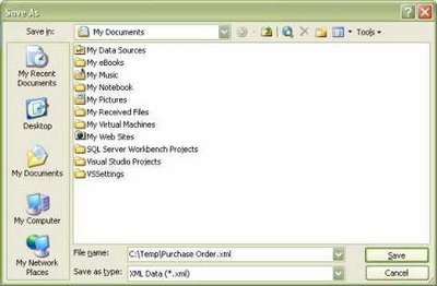
In the Save in box, select the drive or folder path to save the file.
Under the filename box, give a name to the file.Click OK to save the file. Note you must be saving a file in a folder only when you first create it. Once you save it, subsequently the file would be saved in the same location.
All the icons in the Excel Save Dialog is similar to those found in other applications.
You could password protect your files. When saving the file click the the Tools icon and select General Otions. You would be prompted with to enter a password after which your files could be opened only after entering the password. You could also make your files read only by checking the readonly box so that others could see your file but not modfiy it. You could also back it up by checking the create back up button so that you could retrieve the file when you forgot your password. You could also explore the Web Options feature if you like.

Password protecting your file protects your file being modified or looked into by others inside Excel. However it doesn't protect you from someone deleting your files. You may look into Windows sharing to solve this problem

Opening Files
The next step is opening and working with files. The Open Command in Excel is similar to other applications in functioning. You could trigger the Open command by clickingthe open button.
This opens a dialog similar to the save as dialog from which you could select your file to work with and click Open. You could notice a arrow mark to the right of the open button
Clicking this would give you the following options.

• Open - Opens the file
• Open Read-Only - Opens the file in read-only mode.
  You cannot make changes to the file.
• Open as Copy - Opens a copy of the file. Changes you
  make to this file is not reflected in original file
• Open in Browser - Opens the file in a browser
  provided it is a html file(Normal excel files cannot be opened)
• Open and Repair - Opens and repairs the file(This option could be used when Excel terminates suddenly or your data appears garbled)

You could change the default file path of Excel(the default directory when you use the open command).Go to Tools->Options->General and in the Default file location box enter the path of your choice. Quit and restart Excel

Save As
You might face a situation where you would be working on other's file. In such cases, it would be better to save a copy of the original file and work on it instead of actually working in the original file. You can do this by using the Open as Copy option but the problem with this option is that the copy would be saved in the same location of the original file. Thus, if you file is saved in D:\ the copy would also be saved in D:\. To overcome this problem, you could use the Save As option. Go toFile->Save As and follow the procedure you normally do when saving files. Thats it. Save As could also be used to password protect your files when you failed to protect them at the time of creating it.

Save As Webpage
You could also save your excel webpage as an interactive webpage. ClickFile->Save as Webpage. In the dialog box, select your preference to publish either the selected range or worksheet or the entire workbook as webpage and click publish. If you have formulas in the workbook and want to retain them in the webpage, Check the Add Interactivity box. You could change the title that would appear in the webpage in the Change Title box. When you click the Publish box, an another box would appear prompting further changes.

• Under the choose box, select what to publish
• Under the add interactivity box, select spreadsheet
  functionality to preserve you formulas in the webpage.Select pivot table
  functionality to preserve your pivot table in the webpage
• In the title box, enter the title that would be
  displayed in the webpage.
• In the filename box, enter your filename and choose
  where to save
• Check "Autorepublish everytime workbook is saved" box
  to republish your webpage whenever your file is saved.
• Check "Open publish webpage in a browser" to see your
  changes immediately in your default browser
• Click Publish to publish and view your webpage

To disable the autorepublish feature, Goto File->Save as webpage->Publish and then from the choose box, select previously published items and click remove. Normally Excel files aren't saved as webpages. Either they are sent as attachments are viewed in a Excel viewer.

Save as Workspace
Sometimes, you might be working with a particular set of files. Assume you work with 4 sales reports files located in different computers or locations. You may find it embarrasing to open the files every time by going to a specific location. Excel could do this for you. Open all the files you need to work(just for the last time). Go toFile->;Save as Workspace and follow the procedure you normally do when saving files. Thats it, when the next time you open the workspace all the 4 files are automatically opened. If along with those files, other files have opened, close those files and again save the workspace. Take care or else the workspace would be opening too many files for you.

You could open a set of files when you open Excel.Go to Tools->Options->General.In the "At startup ,open all files in" box, enter the path form where you want to open files.Do this with a bit of care as you may end up with a Excel opening a lot of files.Quit and restart Excel

File Search
You could search inside the text of files. Simply Go toFile->File Search and enter the text you want to search and click OK. Files containing the text you enter would show up

Renaming a File
You could rename a file the same way you do with other applications. Sometimes, when you save you may get the following warning message "The following file already exists.Do you want to replace the exisitng file" would be displayed. This is because you are trying to overwrite a file. If you are sure that the old file may be replaced, click YES. Otherwise click NO and save your file under a different name.

Recovering your file
Sometimes when you are working with your file, you may lose it suddenly due to power cuts or sudden termination of Excel. You would really be kicking you as the data you have entered is lost. But its not so. Excel saves everything you type. When you lose your data(you might think you have lost data) suddenly, the next time you open Excel, it displays the list of files you worked but not saved for your review. You could review the files and save them if necessary or discard them.

Autosave files
You could automatically save your files after a specified period of time. This facility is called Autosave. To autosave your files, go to Tools Menu and click Options and select the Save Tab. Under the "Save autorecover info every" box, select the time period to save your files. The default is 10 minutes and don't enter a very small value such as 1 minute as it saves all the open files.See the box is checked and for god's sake, don't uncheck it since it would disable the autorecover feature. Under the "Autorecover save location", enter the location where the files would be automatically saved(This is the location where your files would be temporarily save to recover it in case of sudden termination or computer hangup.After the specified time, it would automatically save in the actual location of the file). The "Disable Autorecover" option is a workbook specific option and can be checked when you don't want to save your workbook automatically. It should be seen that both the autorecover and autosave options are the same and you guessed it right.

Notify files to readwrite
Sometimes when you open a file, you may be prompted with a message that the workbook is being used by an another user.This is because your workbook may be viewed by others. The message would prompt you with three options "Read only","Notify","Cancel".Selecting readonly opens the file to read only, selecting notify notifies you when the other user has closed the file and selecting cancel cancels the operation. When you click notify, you get a notification when the file is closed so that you could read write. It is advised that under such circumstances instead of waiting you Save As the file and work on it.

Sharing your files
The normal rule is that no file can be edited at the same time by more than one user. But in Excel, you may do so. Go toTools->Share Workbook and check the allow changes by more than one user tab. We may see this in detail in a forthcoming post

Know your file
You could know more about your files(though necessarily not) by clickingFile->Properties.
This is just for information purpose.
The File properties have five tabs

• General which gives information about
  • File Name
  • File Size
  • File Type
  • File location
  • Attributes
    
• Summary which gives information about
  • Title
  • Subject
  • Author
  • Keywords
• Statistics which gives information about
  • File created date
  • File modified date
  • File last accessed date
  • File last saved by
    
• Contents which gives information about
  • The worksheets in the workbook and their names
    
• Custom properties that can be set about
  • Name
  • Type
  • Value
  
  

The General,Statistics and Contents are generated by Excel and cannot be changed manually while the Summary and Custom properties are editable. You may use these properties to tell more about your file such as your department, the file content and more but they aren't used commonly.

More file tips

1. You cannot create two files under the same name in a
   single folder. If you need so, you should create a new folder
2. You cannot open two files with the same name at the
   same time. You need to lauch another Excel Application to achieve this.
3. Only one user can edit a file at a time.
4. No changes can be made to a read-only file.
5. You cannot save or rename a file when it is used by
   others.
6. Files are logical devices. No such things really
   exist
7. To give a preview of a workbook as a picture, GotoFile->Properties->Summary and check the Save Preview Picture box.
8. To quickly know the name of the active file type this into a cell =CELL("FILENAME")
9. To know your recent file list, go to files or look into the task pane.

You can increase or decrease the number of recently opened files. To do this, Go to Tools->Options->General. Under the Recently used file list type a number between 1 to 9 and make sure the box is checked

Previous->Getting started with Microsoft Excel
Index->Excel Basic Tutorials
Next->Working with cells

The Edit Menu

Edit

• Undo - Undoes the previous operation - CTRL+Z(You can undo any number of operations until you save the file)
• Redo - Redoes the previous operation - CTRL+Y(You can redo any number of operations that has been previously undone.Redo would not work until an undo operation is done. If no undo operation is done, then Redo repeats the recently executed built-in macro)
• Cut - Performs the cut operation - CTRL+X(Deletes the value from a cell to paste it into other cell)
  
• Copy - Copies the contents of the cell - CTRL+C
  
• Office Clipboard - Displays the office clipboard
• Paste all - Pastes all the items in the office clipboard one after another(When you use this option, the formats would be lost since clipboard is a part of Microsoft Office and not Microsoft Excel)
  
• Clear all - Clears all the collected data in the clipboard
  
• Paste - Pastes the contents into a cell - CTRL+V(The paste operation copies and paste the value of the cell if the content is copied and deletes the value of the cell and pastes it if the cut operation is used. You cannot initiate a paste operation without a cut or copy operation.)
  
• Paste Special... - Pastes the value into the cell in the format and operation you specify
• Paste
• All - Pastes the actual contents into the destination cell(Default)
  
• Formulas - Pastes only the formula (not formats)
  
• Values - Pastes only the values (not formulas and formats)
  
• Formats - Pastes only the formats (not formulas and values)
  
• Comments - Pastes only the comments(not formulas,values,formats)
  
• Validation - Pastes only the validation
  
• All except borders - Pastes everything except the four borders
  
• Column widths - Sets the column width of the destination cell same as that of the copied cell
  
• Formulas and number formats - Pastes formulas and number formats (Number formats refer to format applied to the number such as decimal, percentage etc., This does not include font,color,fill,borders etc.,)
  
• Values and number formats - Pastes values and number formats (not formulas)
  
• Operation
• None - Performs the paste operation(Default)
  
• Add - adds the value of the copied cell to the destination cell(If the value in A1 is 10 and value in A2 is 20, performing this operation replaces the value of A2 as 30(i.e)20+10)
  
• Subtract - adds the value of the copied cell to the destination cell(If the value in A1 is 10 and value in A2 is 20, performing this operation replaces the value of A2 as 10(i.e)20-10)
• Multiply - adds the value of the copied cell to the destination cell(If the value in A1 is 10 and value in A2 is 20, performing this operation replaces the value of A2 as 200(i.e)20*10)
• Divide - adds the value of the copied cell to the destination cell(If the value in A1 is 10 and value in A2 is 20, performing this operation replaces the value of A2 as 2(i.e)20/10)
  

Note: All the above operations are done by appending the value of the copied cell to the destination cell. If you copy A1 with a value of 10 to A2 with a value of 20 and use subtract, A1 is subtracted from A2 and not A2 from A1.If you want this operation to be done, you should copy A2 and paste A1 using subtract

• Skip Blanks - Pastes values in the destination range overriding blanks.
  
• Transpose - Pastes the data of rows to columns and vice versa like a transpose matrix (Pastes the values in the range A1:A10 to A1:J1. Doesn't apply to single cells. Copy and paste area must not overlap)
  
• Paste Link - Creates a link to the original cell so that the value changes each time the source cell is updated.
• Paste as Hyperlink - Pastes a web address as a hyperlink
  

Paste Link is available only when you select All or All except borders.Paste Link always sets an absolute reference if a single cell is selected

• Fill - Fills the value into a cell(Similar to copy operation)

• Down - Fills the value of the cell above into active cell - CTRL+D(Fills the value of cell A1 in A2)
• Right - Fills the value of the cell to the left into active cell - CTRL+R(Fills the value of A1 in B1)
• Up - Fills the value of the cell below into active cell (Fills the value of A2 in A1)
• Left - Fills the value of the cell to the right into active cell (Fills the value of B1 in A1)
• Across Worksheets - Fills the selected cells across all the worksheets selected
• Series - Fills according to the series you specify
• Justify - Justifies the fill operation
• Clear
• All - Clears everthing
  
• Formats - Clears formats only
  
• Contents - Clears contents but keeps formats
  
• Comments - Clears comments only
  
• Delete... - Performs a delete operation
• Delete
  
• Shift cells up
• Shift cells down
• Entire row
• Entire column
  
• Delete Sheet - Deletes the active worksheet
  
• Move or Copy Sheet... - Moves or copies a worksheet
• To book
• Before sheet
• Create a copy
  
• Find... - Searches and finds text or numbers you specity - CTRL+F
• Find What - Enter the text or number to search
  
• Options...
• Format...
• Format - Finds a cell that match the format you specify
  
• Choose format from cell - Pick a cell to search for the format contained in that cell
  
• Clear find format - Clears the format set
  
• Within
• Sheet - Searches the entire sheet(Default)
  
• Workbook - Searches the entire workbook
  
• Search
• By Rows - Searches by rows(1,2,3..... - Default)
  
• By Columns - Searches by columns(A,B,C.....)
  
• Look in
• Formulas - Searches in formulas(Default)
  
• Values - Searches in absolute values(If A1 contains the formula B1+C1 and the result being 12, values return 12 while formulas return B1+C1)
  
• Comments - Searches in comments
  
• Match Case - Performs a case wise search(If the cell value is "ABC" and you search for "abc" then Excel would not find the value you are looking for)
  
• Match entire cell contents - Searches for entire cells (Normally search finds value even it is a part of cell)
  
• Find All - Finds all cells with the specified value.
  
• Find Next - Finds the next cell with the specified value
  
• Replace... - Replaces the existing text with the text you specify - CTRL+H
• Replace With - Enter the text to replace
  
• Options - Same as for FIND
  
• Replace - Replaces the value with the specified value
  
• Replace All - Replaces all the cells that contain the find value with the specified value
  

If you select a single cell for search the entire worksheet would be searched. If you select more than one cell, the specified range would be searched.

• Go To... - Goes to a specified cell or a range you specify - CTRL+G (If you select a single cell and then use GO TO command GO TO searches the entire worksheet. If you select more than one cell, then GO TO command searches only the selected range)
  
• Special...
• Comments - Selects cells with comments
• Constants - Selects cells with absolute value(i.e)cell without formulas
• Formulas - Selects cells with formulas
• Numbers - Selects cells with formulas in numbers(A cell with a formula 10+12)
  
• Text - Selects cells with formulas as text(A cell using "&" sign to join two values or a function that uses a text value)
  
• Logical - Selects cells that hold a logical formula(A cell with any of the following functions: AND,FALSE,IF,NOT,OR,TRUE)
  
• Errors - Selects cells with error values(A cell with an error value such as #N/A,#VALUE etc.,)
• Blanks - Selects cell which has no content in it
• Current Region - Selects the current region for printing
• Current array - Selects the current array that holds an array formula
• Objects - Selects all the objects in the active worksheet. This includes drawing objects, charts and objects inserted using the Insert Menu
• Row differences - All cells that differ from the active cell in a selected row(If more than one row is selected, the comparison is done for each individual row of that selection, and the cell used in the comparison for each additional row is located in the same column as the active cell).
  
• Column differences -All cells that differ from the active cell in a selected row (If more than one column is selected, the comparison is done for each individual column of that selection, and the cell used in the comparison for each additional column is located in the same row as the active cell)
  
• Precedents - Backtraces a formula (If the formula in B1 is A1+A2, then this option selects A1+A2)
  
• Dependents - Select cells that are referenced by formulas.
  
• Direct only - Select cells that are directly referenced by formulas.
  
• All levels - Select cells that are directly or indirectly referenced by formulas (If B1 has the formula A1+A2 and B2 has the formula B1 then if A1 is selected it higlights both B1 and B2 for all levels and B1 for directly only)
  
• Last cell - Selects the last cell that contains formatting.
  
• Visible cells only - Selects cells visible for printing(Does not select hidden rows or columns)
  
• Conditional formats - Selects cells that contain conditional formats
  
• Data Validation
• All - Selects cells that contain data validation.
  
• Same - Selects cells that contain same data validation as the cell selected.
  

• Links - Opens the EDIT WORKBOOK LINKS dialog to edit formula links contained in other workbooks
• Update Values - Updates the values in the active workbook(if any change has been made in the source workbook)
  
• Change Source - Changes the source of the links(i.e.)worbooks(If Book2 contains references from Book1 and you want link Book2 to Book3 instead of Book1, you should use this option.This substitutes the links of Book1 with Book3.So if your link in Book2 is ='[Book1.xls]Sheet1'!A1 then it would change to ='[Book3.xls]Sheet1'!A1
  
• Open Source - Opens the source workbook that links to the active workbook(if it is not open)
  
• Break Links - Replaces all the formulas with values and break links with the source workbook
  
• Check Status - Checks the status of the source book and displays the status such as OK, Source opne etc.,
  
• Startup Prompt - Determines the message to be displayed when a user opens a workbook that have external references
  
• Lets users choose to display the alert or not - Prompts the user with a dialog box to edit external references.
  
• Don't display the alerts and don't update automatic links - Opens the workbook without prompting the users and without updating values.
  
• Don't display the alert and update links - Opens the workbook without prompting the users but updates the values.
  
• Update
  
• Automatic - Automatically updates the workbook(Default option unless it is set to manual in the Tools->Options->Calculation tab)
  
• Manual - Manually updates the workbook
  
• Object - Edits the object selected. Objects here means a different application such as Microsoft Word, AutoCAD MS Map embedded in excel using the Insert->Object option in the Insert Menu. This doesn't mean drawing objects created using excel.

Previous->The File Menu Index->Menus and Toolbars Next->The View Menu

The File Menu

File

• New->Creates a new file->Ctrl+N
• Open->Opens a new file->Ctrl+O
• Close->Closes the active file->Ctrl+W(Hold down shift and then click file to close all open files)
• Save->Saves the active file->Ctrl+S(This action only saves the active file, not all open files)
  
• Save As->Saves the file in the required format(You could use this option to save files in any previous format or a lotus file or a CSV file or any other format you want.The default option is to save the workbook as Microsoft Excel file.Remember if you use this option you may lose certain features of Excel if you save in an another format)
  
• Save As Web Page->Saves the file as webpage(If you have used buil-in functions,links to other workbooks,pivot tables then they may not work in webpage.The file is saved as a webpage with an embedded spreadsheet)
  
• Save Workspace->Saves all open files under one name(If you have 4 open files and you would be always working with the 4 files you may save them as workspace.Whenever you open the workspace,all the 4 files are opened)
  
• File Search->Performs a file search operation.Searches text within files
• Web Page Preview->Previews how your excel file would look as a webpage.Shows only static text and formatting.
• Page Setup->Opens the Page Setup dialog box used for printing.
• Print Area
• Set Print Area->Sets the print area for the selected range of cells. By default, excel sets the print area beginning from the first cell to the last cell that have content in it.
  
• Clear Print Area->Clears the print area already set(Mostly by selecting the set print area option)

• Print Preview->Previews how the document would be printed.
• Print->Opens the Print Dialog Box->Ctrl+P
• Send To(Relates to Microsoft Outlook,Outlook Express)
  
• Mail Recipient->Sends the worksheet content as an e-mail
• Mail Recipient(for Review)->Emails the workbook for reviewing(the workbook must be shared to use this option)
  
• Mail Recipient(as Attachment)->Emails the entire workbook as an attachment
• Routing Recipient->Emails the workbook from within Excel instead of Microsoft Outlook
  
• Exchange Foler->Places the workbook in any folder of your default mail client(If you use Microsoft Outlook,you may send a workbook directly to inbox)
• Online Meeting Participant->Shows you online meeting status and more scheduled by NetMeeting
• Recipient using Internet Fax Service->Faxes you workbook
  
• Properties->Shows the properties of the active file
• Recently Opened files->Shows the list of recently opened files(1 to 9 as in Tools)
• Exit-Quits Microsoft Excel